MIT线性代数笔记Unit1

Unit I: $Ax = b$ and the Four Subspaces

1 The Geometry of Linear Equations（线性方程组的几何解释）

The geometric picture of a matrix’s column space is the first key idea of linear algebra.

Row Picture

线性方程组的解是函数图像的交点

Column Picture

$Ax=b$，$b$为$A$列向量的线性组合（linear combination of columns）

线性方程组的解是列向量的线性组合系数

Matrix-Vector Multiplication

两种计算方法：

• row way 矩阵各行与向量之间的点乘

• column way 矩阵各列以向量为系数的线性组合

2 Elimination with Matrices（矩阵消元）

Elimination is the technique most commonly used by computer software to solve systems of linear equations.

Elimination

利用每行的主元消元+回代（eliminate with pivot and back substitution）

Elimination Matrices

利用矩阵乘法来描述消元法——变换矩阵：

• 左乘行变换（左乘将矩阵的行向量进行线性组合）

• 右乘列变换（右乘将矩阵的列向量进行线性组合）

3 Multiplication and Inverse Matrices（乘法和逆矩阵）

Once we have used Gauss’ elimination method to convert the original matrix to upper triangular form, we go on to use Jordan’s idea of eliminating entries in the upper right portion of the matrix.

Matrix Multiplication

$AB=C$几种计算方法：

• Standard (row times column) 行乘列计算每个元素：$c_{ij}=row_{i}(A)\cdot col_{j}(B)$

• Columns $A$列向量的线性组合的拼接

• Rows $B$行向量的线性组合的拼接

• Column times row 列乘行的和：$C=\Sigma(col_{i}(A)\cdot row_{i}(B))$

• Blocks 分块乘法

Inverse

• Invertible, non-singular —— $A^{-1}A=I$

• Singular —— No inverse 充要条件：存在$x\neq 0$使$Ax=0$（反证）

• 求解$A^{-1}$：Guass-Jordan Elimination —— 通过行变换消元将$[A,I]$变换为$[I,A^{-1}]$（变换矩阵$E[A,I]=[EA,EI]$，由于$EA=I$，所以$E=A^{-1}$，所以$EI=A^{-1}$）

• $(AB)^{-1}=B^{-1}A^{-1}$（ps：有趣的例子，先穿袜子再穿鞋的逆是先脱鞋再脱袜子hhh）

• $(A^T)^{-1}=(A^{-1})^T$

4 Factorization into $A = LU$（矩阵的LU分解）

If there are no row exchanges, the multipliers from the elimination matrices are copied directly into $L$.

$A = LU$

可以使用消元法将矩阵$A$变换为上三角矩阵$U$（upper triangular），$EA=U$，由此可以得到$A=LU$，$L$作为变换矩阵$E$的逆，是一个下三角矩阵（lower triangular），且各行主元均为1

$A=LU$这种表示方法相较于$EA=U$的优越性：如果没有换法变换，高斯消元过程中的消法变换的乘数会在$L$中直观地显示（由于消元过程自上而下，在$E$中，先进行的消法变换，会改变尚未进行以该行主元进行消法变换的行，以至于消法的乘数在$E$中会产生叠加的效果，而$L=E^{-1}$，自下而上，不会产生乘数的叠加效果，原始的乘数会在$L$中直观地显示出来）

How expensive is elimination?

即计算$A=LU$的时间$\approx1^2+2^2+\cdots+(n-1)^2+n^2=\sum_{i=1}^ni^2\approx\int_0^nx^2dx=\frac{1}{3}n^3$

Row exchanges

行换法变换 —— 置换矩阵（permutation matrix）$P$

• $P^{-1}=P^T$

• $n$阶置换矩阵有$n!$个，乘法运算封闭，构成乘法群（multiplicative group）

5 Transposes, Permutations, Spaces $R^n$（转置，置换，向量空间）

If a collection of vectors is closed under linear combinations, and if multiplication and addition behave in a reasonable way, then we call that collection a vector space.

Permutations

考虑换法变换后，LU分解变为：$PA=LU$，$P$为置换矩阵

对于任意可逆矩阵，都可以对其进行LU分解表示 —— $PA=LU$

Transposes

• $\left(A^{T}\right)_{ij}=A_{ji}$

• 对称矩阵（symmetric matrix）—— $A=A^T$

• $A^TA$ is always symmetric

• $(AB)^T=B^TA^T$

Vector spaces

• 向量空间：对线性组合运算封闭（加法与数乘）

• $R^n$ —— 所有$n$维向量张成的空间

• 子空间（subspace）

  • $R^2$的子空间：$R^2$，所有过原点的直线，0向量

  • $R^3$的子空间：$R^3$，所有过原点的平面，所有过原点的直线，0向量

• 矩阵张成的列空间：包含矩阵的所有列向量以及它们的线性组合

• 两个子空间的交集仍构成子空间

6 Column Space and Nullspace（列空间和零空间）

“We only live so long, we just skip that proof.”

Column space

$Ax=b$有解 充要条件：$b$在$A$的列空间中

Nullspace

矩阵$A$的零空间：包含$Ax=0$的所有解向量

注：$Ax=b,b\neq0$的解空间是不过原点的点/直线/平面，不构成子空间

列空间和零空间是由方程组构筑子空间的重要方法

7 Solving $Ax = 0$: Pivot Variables, Special Solutions（求解$Ax = 0$：主变量，特解）

The rank $r$ of $A$ equals the number of pivot columns, so the number of free columns is $n − r$: the number of columns (variables) minus the number of pivot columns. This equals the number of special solution vectors and the dimension of the nullspace.

Computing the nullspace

利用消元法求解方程组（原理：消元法只改变列空间，不改变解空间）

消元后得到阶梯形矩阵（echelon），可以找出pivot columns和free columns，矩阵$A$的秩（rank）等于它包含的主元（pivots）个数

Special solutions

free columns对应的变量为自由量（free variables），通过给自由量任意赋值，可以求得方程组的特解

$A$的秩$r$等于pivot columns的数量，所以free columns的数量为$n-r$，这也等于特解的数量及其解空间的维度

Reduced row echelon form

利用回代的方式继续向上消元可以得到行最简型矩阵（reduced row echelon），即主元均为1，且主元所在列其他元素均为0

通过一些列交换，行最简型矩阵可以变换为 $R=\begin{bmatrix} I & F \\ 0 & 0 \end{bmatrix}$ ，此处$I$是一个$r$阶单位方阵，对应着pivot columns；则零空间矩阵为$N=\begin{bmatrix} -F \\ I \end{bmatrix}$，此处$I$是一个$n-r$阶单位方阵，$RN=0$，$N$的各列即为方程组的各特解

8 Solving $Ax = b$: Row Reduced Form $R$（可解性和解的结构）

If a combination of the rows of $A$ gives the zero row, then the same combination of the entries of $b$ must equal zero.

Solvability conditions on $b$

之前提到$Ax=b$有解 充要条件：$b$在$A$的列空间中

另一种等价的描述方式 —— 如果$A$中的某种行的线性组合为零行，则$b$中元素相同的线性组合结果为0（如果$A$中的行被消元为零行，$b$中对应的元素也被消元为0）

Complete solution

• 一个特解（particular solution）—— 令所有自由量都为0，解出该特解$x_p$

• 零空间（nullspace）—— 求解$Ax=0$，解出零空间$x_n$

• $x_{complete}=x_p+x_n$

Rank

• 列满秩（Full column rank）无自由量，零空间只有0向量，$Ax=b$如果有解则仅有唯一解$x_p$

• 行满秩（Full row rank）每行都有主元，消元不会出现零行，$Ax=b$必有解

• 满秩（Full row and column rank）可逆矩阵，零空间只有0向量，$Ax=b$必有解则仅有唯一解$x_p$

$$\begin{array}{|c|c|c|c|c|c|}\hline\text{$A\in R^{m\times n}$}&r=m=n&r=n<m&r=m<n&r<m,r<n\\\hline\\R&I&\left[\begin{array}{cc}I\\0\end{array}\right]&\left[\begin{array}{cc}I&F\end{array}\right]&\left[\begin{array}{cc}I&F\\0&0\end{array}\right]\\\\\#\text{solutions to $Ax=b$}&1&0\text{ or }1&\text{infinitely many}&0\text{ or infinitely many}\\\hline\end{array}$$

9 Independence, Basis, and Dimension（线性相关性，基，维数）

If the columns of $A$ are independent then all columns are pivot columns, the rank of $A$ is $n$, and there are no free variables.

Linear independence

向量间线性无关：不存在非0系数使向量的线性组合为0

如果矩阵的列向量线性无关，则其方程组无自由量，零空间只有0向量

Basis and dimension

向量空间的基：线性无关且能够生成该空间的一组向量

对于一个向量空间，它的基向量数量一定，该数量即为该空间的维数$dim$

• 列空间的维数 = 矩阵的秩$r$

• 零空间的维数 = 自由量的数量 = $n-r$

10 The Four Fundamental Subspaces（四个基本子空间）

The left nullspace is the collection of vectors $y$ for which $A^Ty = 0$. Equivalently, $y^TA = 0$; here $y$ and $0$ are row vectors. We say “left nullspace” because $y^T$ is on the left of $A$ in this equation.

Four subspaces

$A\in R^{m\times n}$

• 列空间（Column space），$C(A)\in R^m$，$dim=r$，基为pivot columns

• 零空间（Nullspace），$N(A)\in R^n$，$dim=n-r$，基为free columns

• 行空间（Row space），$C(A^T)\in R^n$，$dim=r$，基为消元后的非零行（注：消元时只改变了列空间，而行空间不变，故行空间的基会在消元后直接呈现出来）

• 左零空间（Left nullspace），$N(A^T)\in R^m$，$dim=m-r$，基为消元后$R$中零行对应的变换矩阵$E$中的行向量（计算方法：$EA=R$，将$[A,I]$变换为$[R,E]$，由此求出变换矩阵$E$，根据$R$中的零行找出$E$中对应的行向量即为左零空间的基 —— $y^TA=0$）

New vector space

将矩阵看作向量，方阵也可以构成向量空间（加法、数乘封闭）

一些矩阵子空间：

• 所有上三角矩阵（upper triangular matrices）

• 所有对称矩阵（symmetric matrices）

• 所有对角矩阵（diagonal matrices）

11 Matrix Spaces; Rank 1; Small World Graphs（矩阵空间，秩1矩阵，小世界图）

“What’s Hillary’s distance to Monica? I don’t think we’d better put that on tape here. That’s one or two, I guess.”

New vector spaces

很多不是向量的元素，也可以看作是向量，构成空间

• 3阶方阵（3 by 3 matrices）

  • 所有3阶方阵构成空间$M$，$dim(M)=9$

  • 所有3阶上三角矩阵构成空间$U$，$dim(U)=6$

  • 所有3阶对称矩阵构成空间$S$，$dim(S)=6$

  • 所有3阶对角矩阵构成空间$D=U\cap S$，$dim(D)=dim(U\cap S)=3$

  • $U$和$S$子空间的和构成空间，包含所有取自$U$和$S$的元素的可能和，此空间就是$M$，$dim(U+S)=dim(M)=9$

  • $dim(U)+dim(S)=dim(U+S)+dim(U\cap S)$

• 微分方程（Differential equations）

  • 齐次线性微分方程的所有解构成子空间 —— 零空间

• 一个例子：在$R^4$中，所有满足$v_1+v_2+v_3+v_4=0$的向量$\begin{bmatrix} v_1 \\ v_2 \\ v_3 \\ v_4 \end{bmatrix}$构成子空间，$dim=3$（从该空间为矩阵$A=\begin{bmatrix} 1&1&1&1 \end{bmatrix}$零空间的角度思考，$A$的秩为1，列空间的维度为1，则零空间的维度为4-1=3，另外，行空间的维度为1，左零空间的维度为0，仅有零元素）

Rank one matrices

秩1矩阵都可以表示为$A=UV^T$，$U$和$V$都是列向量

Small world graphs

图$G=\{nodes, edges\}$，可用来描述人际关系等

六度分隔（six degrees of separation）

使用矩阵来描述图，以解决实际问题

12 Graphs, Networks, Incidence Matrices（图和网络）

When we use linear algebra to understand physical systems, we often find more structure in the matrices and vectors than appears in the examples we make up in class. There are many applications of linear algebra; for example, chemists might use row reduction to get a clearer picture of what elements go into a complicated reaction.

Incidence matrices

对于一个有$n$个结点，$m$条边的有向图，其关联矩阵每列对应一个结点，每行对应一条边，边出点处的值为-1，边入点处的值为1，其他位置处的值为0，关联矩阵是稀疏的（sparse）

图中的环（无向环loops）对应着关联矩阵中的线性相关，无环图是树

如果图表示电势图，每个结点处有一个电势值，边代表了电流流向（电势差的方向），关联矩阵为$A$，则有以下关系：

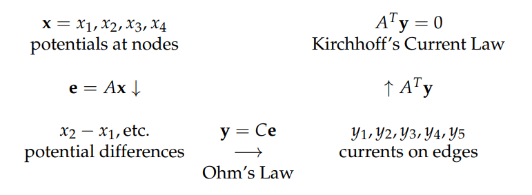
通过关联矩阵，串联起了两点间电势差的计算和基尔霍夫电流定律的求解，如果存在外部电流源，则基尔霍夫定律可以写为$A^Ty=f$，$f$为引入的外部电流，由此得到基本平衡方程 —— $A^TCAx=f$

对于连通图，关联矩阵的秩为$n-1$，即支撑树的边数，由此可以得出$\#nodes-\#edges+\#loops=1$，串联起了零维的点、一维的线、二维的回路（区域、面），即为欧拉公式（利用线性代数实现了欧拉公式的推导）

13 Quiz 1 Review（复习一）